Part 1 Review

Optical Fiber: The Key to High-Speed Digital Transmission

Current State

In today’s interconnected world, high-speed data transmission is essential. Optical fiber technology, developed over the past 40 years, plays a critical role in enhancing transmission line performance and reliability, especially in digital video transmissions. Leading manufacturers continually push the boundaries of data rates and distance applications, ensuring thorough testing and support for improved product performance.

Optical Fiber’s Future

The demand for fast and reliable data transmission is growing, driven by activities like streaming, gaming, and telemedicine. Achieving and maintaining high-speed data involves technological advancements, infrastructure development, and regulatory updates. Significant milestones include the transition from dial-up to broadband, fiber-optic networks, and the evolution of 4G LTE and 5G technologies. To carry these high data rates, copper wire and optical fiber are essential, with optical fiber being the primary choice for distances over 1-2 meters.

Understanding Optical Fiber

Optical fiber’s capabilities are rooted in Snell’s Law, governing the refraction and total internal reflection of light. Historical experiments by Colladon and Babinet in the 19th century laid the groundwork for guiding light through optical fibers.

20th Century Advances

The 20th century saw major advancements in fiber optics, particularly through the work of Kuen Kao, who significantly reduced signal loss in optical fibers. By the 1970s, technological breakthroughs made fiber-optic communication commercially viable.

Material Evolution

The evolution of optical fiber materials has been driven by the quest for better performance. From early experiments with glass and water, researchers developed high-purity silica glass fibers in the 1960s, leading to low-loss fibers. Subsequent innovations include plastic optical fibers, photonic crystal fibers, and nanotechnology-based materials.

Single-Mode and Multi-Mode Fibers

Optical fibers are categorized into single-mode and multi-mode types, each with specific applications. Single-mode fibers offer high bandwidth and long-distance transmission, essential for telecommunications and internet backbones. Multi-mode fibers, with larger core diameters, are suitable for short-distance applications like local area networks and data centers.

Future Perspectives

The future of optical fiber technology is promising, with ongoing research aimed at enhancing performance and functionality. Optical fibers will continue to play a crucial role in high-speed communication networks, data centers, 5G networks, and medical imaging.

communication networks, data centers, 5G networks, and medical imaging.

Moving Forward Into Optical Fiber Hardware

Making the Fiber Connection

Optical fiber coupling with light emitters is a critical aspect of fiber optics communication and various applications where efficient transfer of light from any form of emitter into an optical fiber is required. Here are a few examples of how this mechanical coupling can takes place. Light-emitting diodes (LEDs) generally have either an edge-emitting or surface-emitting structure, each necessitating different methods for coupling into optical fibers Fig 1. 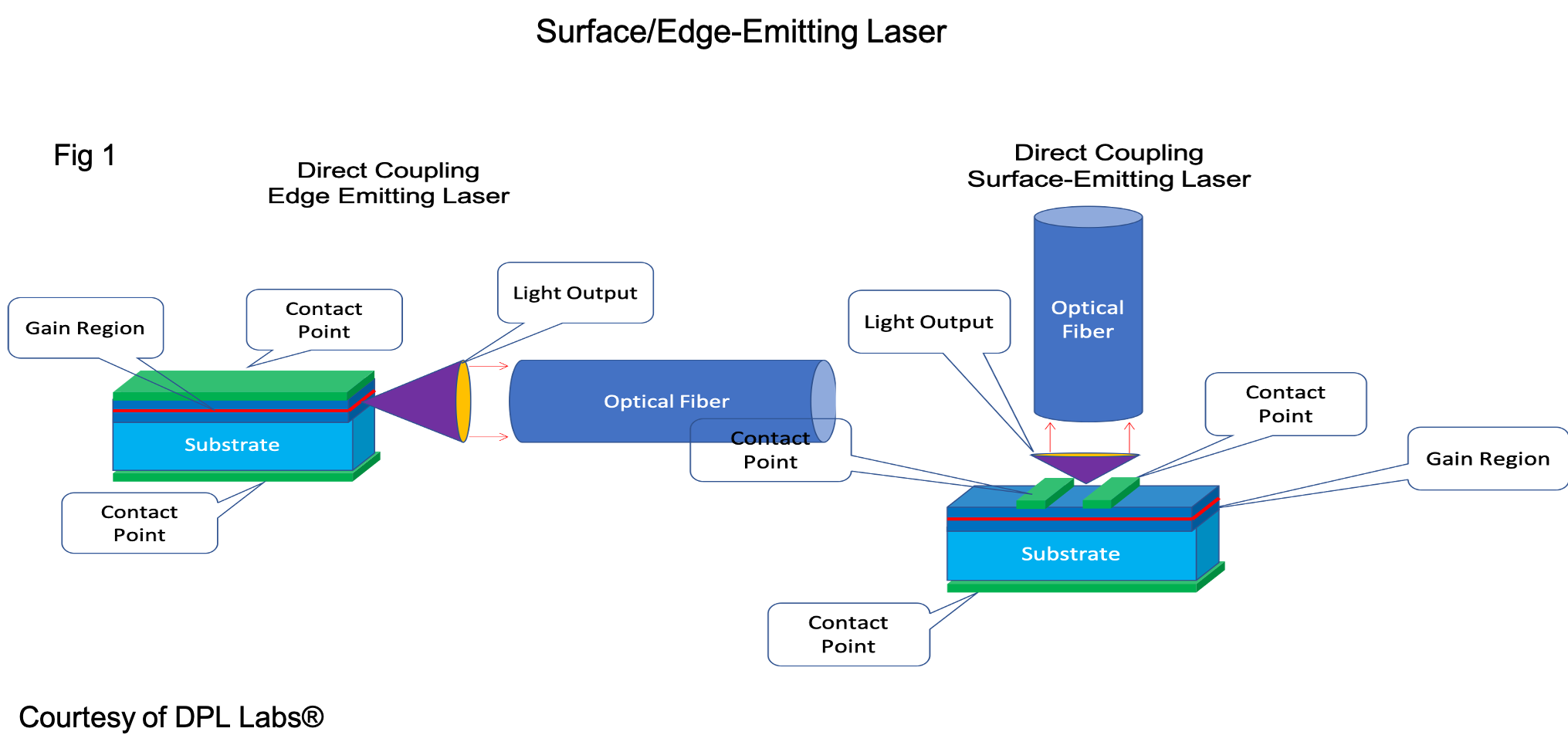This distinction is especially significant in fiber optic communication systems, which employ specific types of surface-emitting LEDs (known as SLEDs) and edge-emitting LEDs (known as ELEDs). However, this division is not unique to fiber optic communications and applies to most other LEDs as well.

Direct Coupling Using LEDs

The simplest form of coupling is direct coupling as the name suggests it. Each fiber is positioned directly in front of its emitter’s face. It provides a straightforward application by placing the end of an optical fiber directly against the face of its emitter. Not much rocket science here.

Advantages:

• By far the simplest process for coupling

• Relatively easy to align

• Minimal components needed

• The least amount of cost

Disadvantages:

• Low performance due to a high probability of misalignment

• Extremely sensitive to positional changes

• High probability of thermal expansion

Applications:

• Short-distance communication links

• Low-cost consumer electronics

Lens Coupling

Description: Lenses are used to focus the light with pinpoint accuracy from the emitter into the optical fiber. This can involve various types of lenses such as spherical, aspherical, or GRIN (graded-index) lenses. These lenses are used for laser-to-fiber, fiber-to-fiber, and fiber-to-detector couplings.

Advantages:

• Higher coupling efficiency by focusing light directly into an optical fiber

• Better control over the beam’s profile and divergence

Disadvantages:

• Increased complexity in alignment

• Increased placement time

• Additional optical components increase cost and potential losses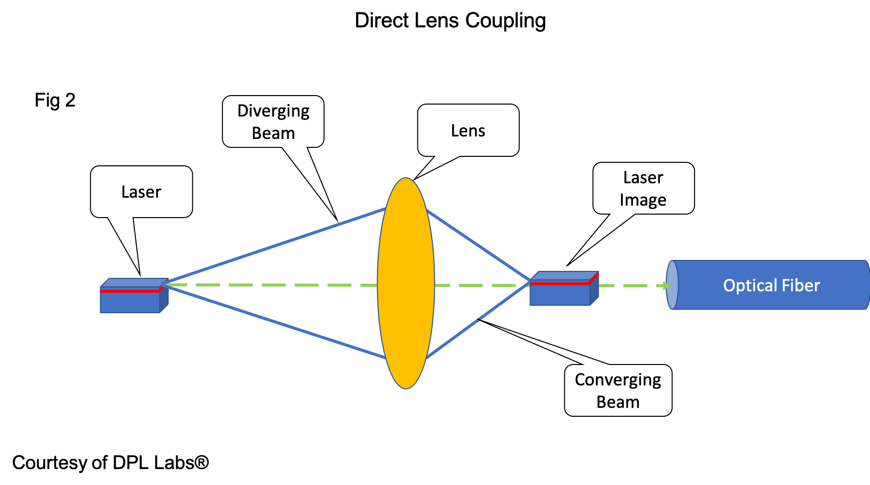

Fiber End-Face Shaping

Description: Shaping the end-face of the fiber (e.g., angling, tapering, or microlens integration) to improve coupling efficiency.

Advantages:

• Customization for specific applications

• Potential for high efficiency without additional components

Disadvantages:

• Requires precise manufacturing techniques

• Potential for higher initial setup costs

Microlenses on Emitters

Description: Microlenses are directly fabricated on the surface of the emitters to collimate or focus the emitted light.

Advantages:

• Compact design

• Improved coupling efficiency by directly shaping the emitter’s output

Disadvantages:

• Complex fabrication processes

• Difficulty integrating with all types of emitters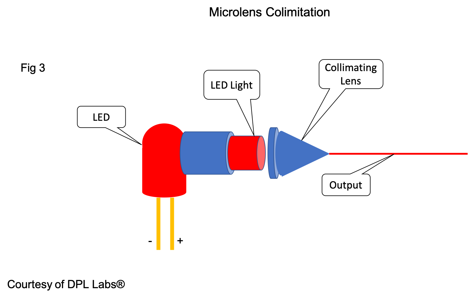

Waveguide Coupling

More widely used for RF communications, waveguides can also be effectively used for fiber transmissions. For RF, a waveguide is a rectangular, circular, or oval “pipe” filled with air or dielectric material, designed to convey RF energy. The structure’s physical design dictates the frequencies it can transport. While many different modes are possible, the lowest order mode is typically used.

Integrated optics utilize waveguides for the transmission of light, where light propagates within a waveguide medium with a higher refractive index than the surrounding material, allowing for low-loss propagation. This ability to guide light as a trapped wave within a waveguide is the fundamental principle of integrated optics, similar to fiber optics. In this context, various circuit devices such as lasers, modulators, and detectors can be fabricated within the same material as the waveguide and directly coupled into it. The waveguide and associated devices can be made very small, enabling close packing of many devices. This concept leads to the creation of electro-optic integrated circuits (EOICs). The integrated optics approach results in compact, durable devices that can be easily and cost-effectively manufactured. Unlike atmospheric light propagation, integrated optics avoids variations and losses caused by atmospheric conditions, offering advantages in size and cost efficiency.

Description: Integrated optical waveguides are used to direct the light from the emitter into the optical fiber.

Advantages:

• High coupling efficiency and stability

• Suitable for integrated photonic circuits

Disadvantages:

• Complex fabrication and alignment

• Higher cost and design effort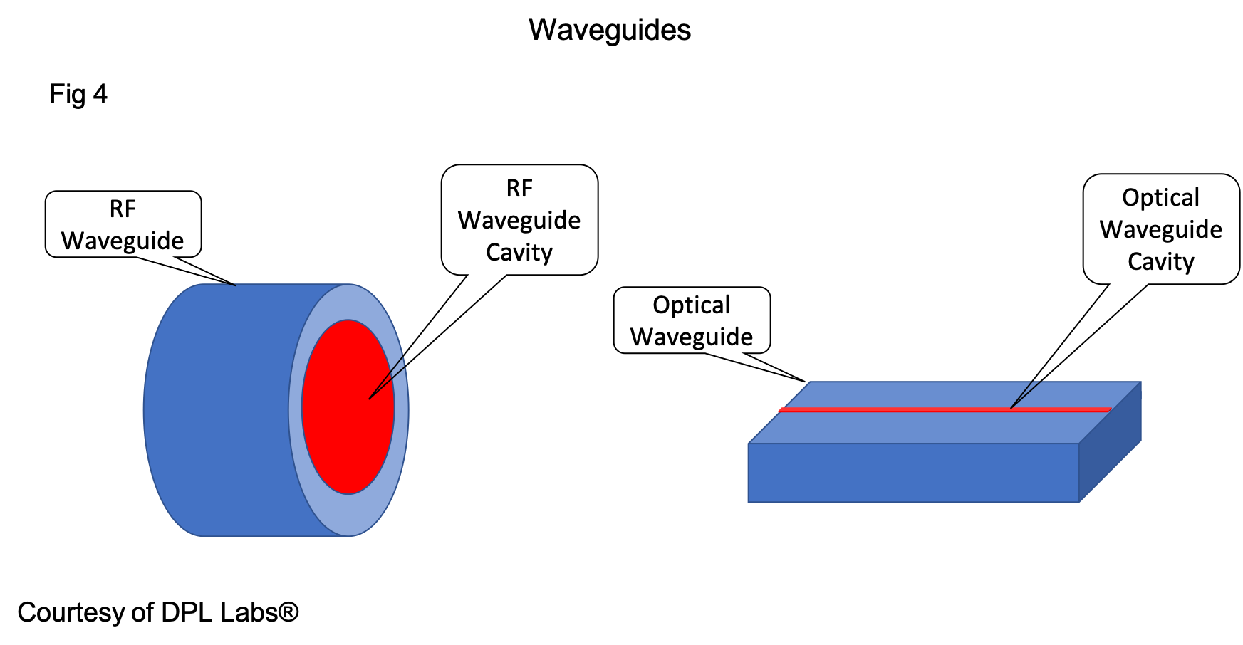

Fast Forward to the VCSEL

Vertical Cavity Surface-Emitting Laser

A VCSEL (Vertical Cavity Surface-Emitting Laser) is a type of semiconductor laser diode that emits light vertically through the devices top surface, as opposed to edge and surface-emitting lasers that emit light from the side. VCSELs are widely used in a variety of applications, including data communication, sensing, and laser printing.

Structure:

• Active Region: The active region of a VCSEL is typically composed of quantum wells where electron-hole recombination occurs to generate photons.

• Distributed Bragg Reflectors (DBRs): VCSELs utilize DBRs above and below the active region to form the optical cavity. DBRs are composed of multiple alternating layers of materials with different refractive indices, creating a high reflectivity mirror.

• Oxide Layers: These layers are often used to confine the current and optical modes, improving efficiency and performance.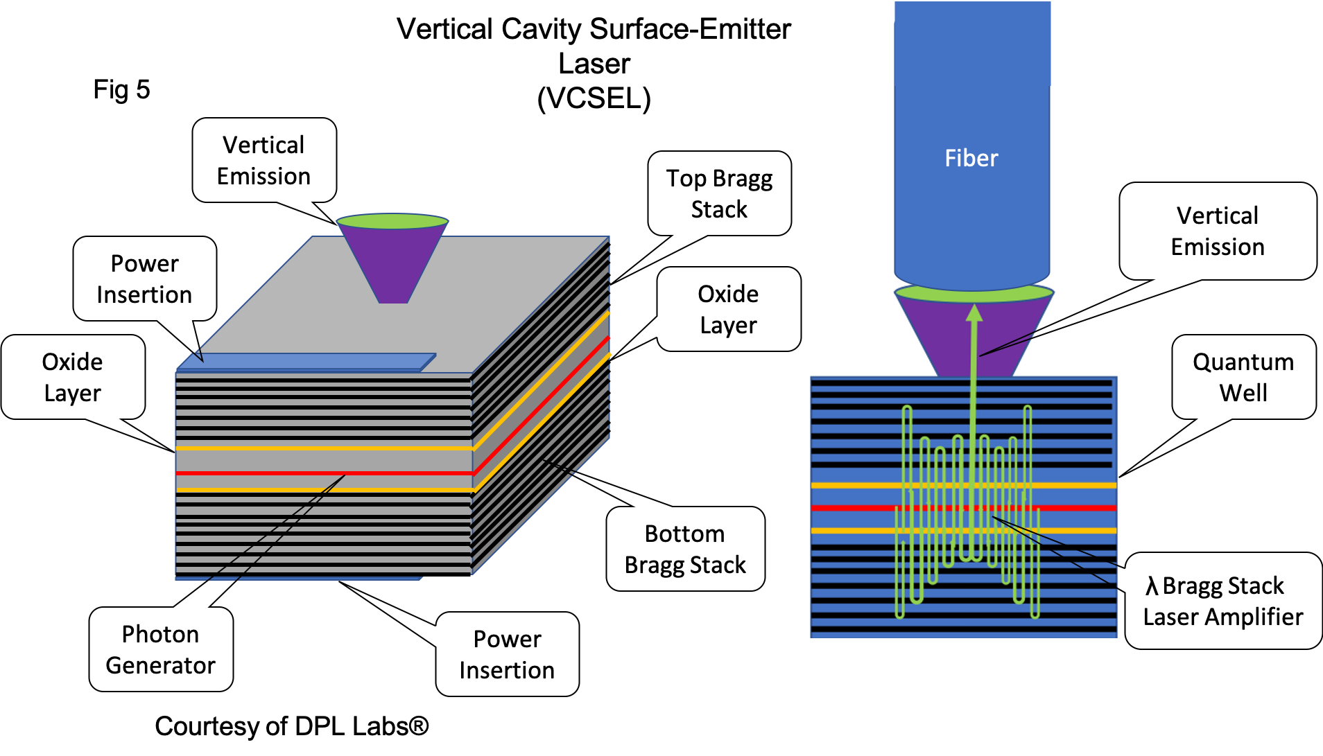

Operation Principle:

1. Electrical Injection: Current is injected the power pad electrodes.

2. Photon Generation: Electrons and holes recombine in the quantum wells, producing photons.

3. Optical Cavity Resonance: The generated photons are reflected back and forth between the matched Wavelength-Distributed Bragg Reflectors. This induces a photon resonance, form of light amplifier within the quantum wells.

4. Quantum Well: The Bragg Generator goes viral increasing its optical output.

5. Bragg Stack Mirror: Generates photon regeneration building to better than 90% of its laser output compared to typical laser diodes outputs of 20% to 30% output.

6. Vertical Emission: The resonant light builds up in intensity and is emitted vertically through the top DBR.

Advantages:

• Efficiency: High efficiency due to low threshold currents and high differential efficiency.

• Beam Quality: Produces a circular beam with a low divergence angle, not requiring any lens and making it easy to couple with reflective coupling into optical fibers.

• Scalability: Easily scalable to arrays, allowing for multiple VCSELs with high-density integration in applications like data communication.

Applications:

• Data Communication: Widely used in optical fiber communication systems for high-speed data transfer.

• Consumer Electronics: Replacing ancient copper transmission lines.

• Sensing: Employed in various sensing applications, including LIDAR (Light Detection and Ranging) for autonomous vehicles and biometric sensors.

• Laser Printing: Used in laser printers and scanners for high-resolution printing.

Key Technical Specifications:

• Wavelength: Common wavelengths include 850 nm for data communication and sensing, with other wavelengths tailored for specific applications.

• Output Power: Typically ranges from a few milliwatts to several tens of milliwatts, depending on the application.

• Modulation Speed: Can achieve high modulation speeds, making them suitable for gigabit and terabit data transmission.

VCSEL technology has revolutionized various industries with its unique properties, offering high efficiency, excellent beam quality, and the ability to form dense arrays. Consumer electronics now have the pathway to affordable optical fiber transmission, offering state-of-the-art technology over extreme distances. As technology advances, VCSELs continue to find new applications and improve the performance of existing systems.

So, where are we going with all this?

Even with this relatively brief abstract highlighting Optical Fiber’s history and advancements, one might think it epitomizes performance and reliability. However, as optical fiber entered the consumer space, interoperability issues arose while marketing continued to deliver excessive grandstanding and claims that echoed its historical success. So, what happened, and why can’t we rely on an optical transmission line with a history of significant advancements?

There is no doubt that the most widely used consumer application of optical fiber today is digital video. Video studios can fully utilize these devices, but the scale of their usage is minuscule compared to what is needed for consumer video. In this context, tens of millions of devices are designed and manufactured, primarily in the Far East. Does this geographic detail matter? In reality, it does not. Regardless of whether they are built in Antarctica or Taiwan, manufacturing technology is available. Therefore, the issue must lie deep into the bowels of these transmission lines.

When designing a product, an engineer must have a comprehensive understanding of the product being created. The competition is fierce, with millions of players vying to outsell each other. In my opinion, it is crucial to develop a deep familiarity with each type of transmission and its composition. Digital video designs are frequently updated. Take HDMI for example, with increasing data rates, new revisions appear unexpectedly with and in-field failures that often go unreported. In this advanced area of technology, both manufacturers and engineers must thoroughly understand every aspect of the transmission line they are designing. One of my professors once said, “To truly understand something, you must wear it like a shirt.” This means that if my shirt is too tight, its sleeves are too short, or its collar is too tight, I notice it immediately. Unfortunately, we aren’t seeing this level of awareness and empathy. Instead, numerous issues are surfacing almost daily.

Overall Dynamic Range

You need to step back and take in the entire landscape. First, the signal to be transmitted must be converted into light energy. We’ve covered this before, but let’s review it briefly to ensure clarity. Figure 6 shows a direct-coupled emitter configuration. Digital modulation enters and is converted into light energy, using a high signal as an ON state and a low signal as an OFF state. This configuration is referred to as a non-inverting signal signal device, where the polarity of the input data matches the output data. This process is straightforward, so we’ll stick with it.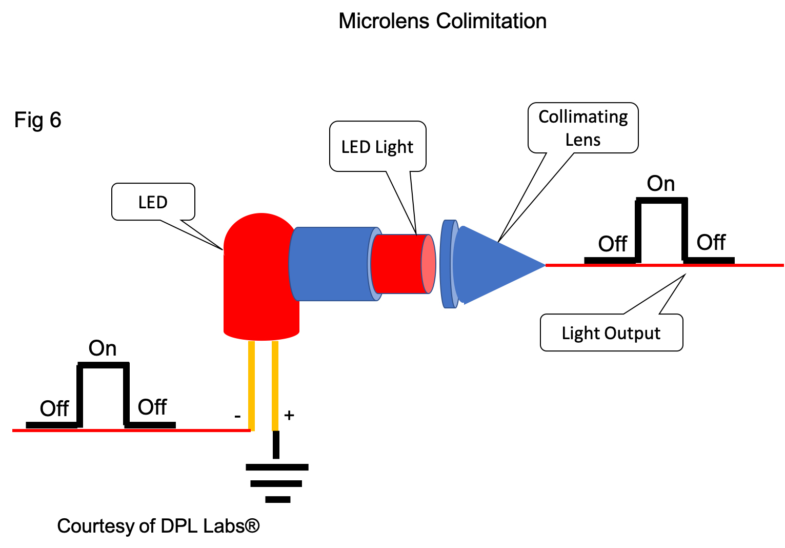

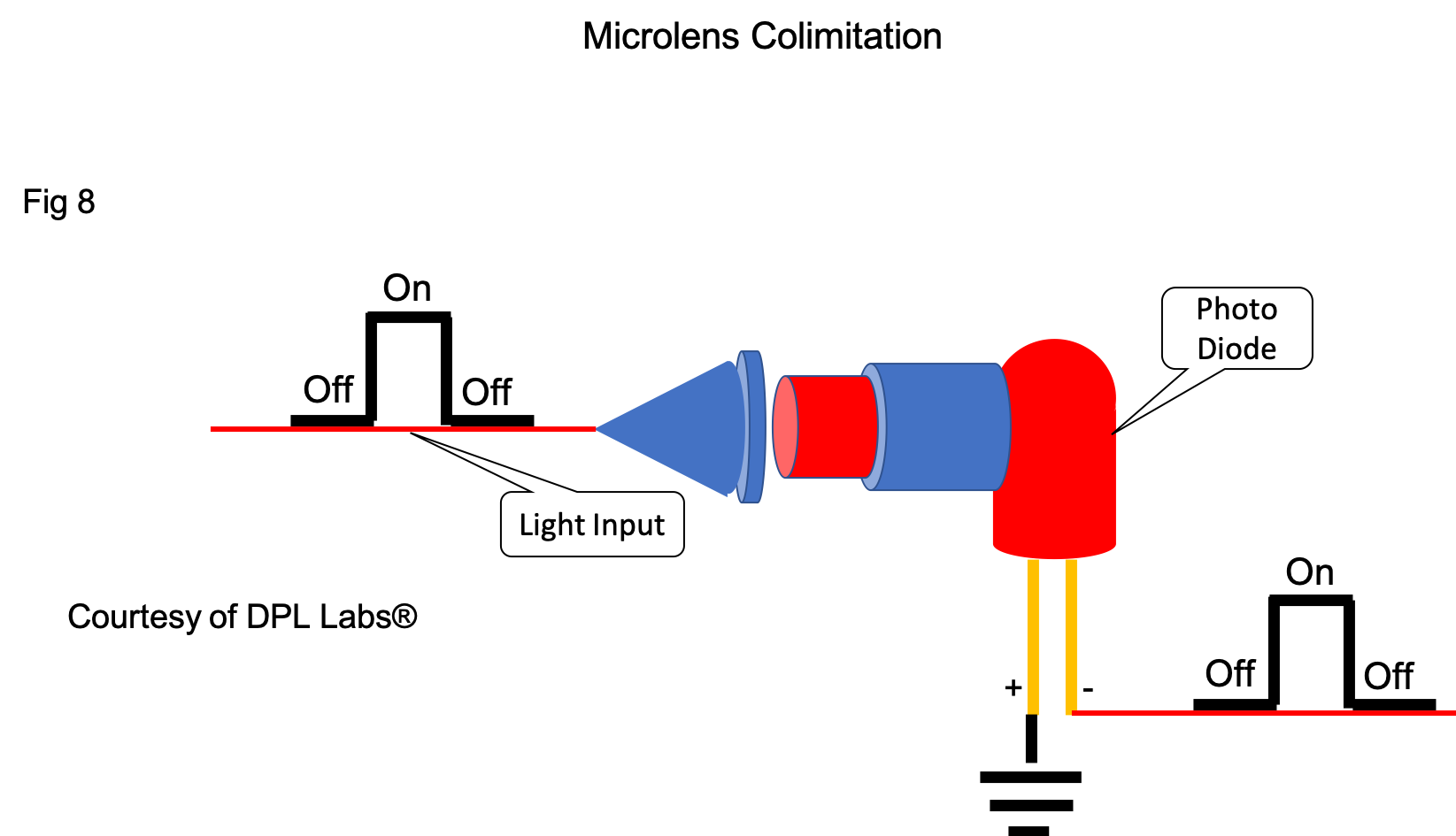
The first question that arises is what is the ON threshold that turns on the LED, and what is the OFF that deactivates it? Each emitters characteristic has specific points within its specifications that dictate this, as shown in Figure 7. LEDs do not necessarily have an abrupt on-and-off state, so engineers must account for these values when developing any optical transmitter. In reality, it is a bit more complex, but for illustration purposes, Fig 7 should convey the basic idea. Once these levels are determined, a similar strategy must be applied to the receiving side of the transmission line, as illustrated in Figure 8. As long as all specifications align with the entire interface, everything should function correctly.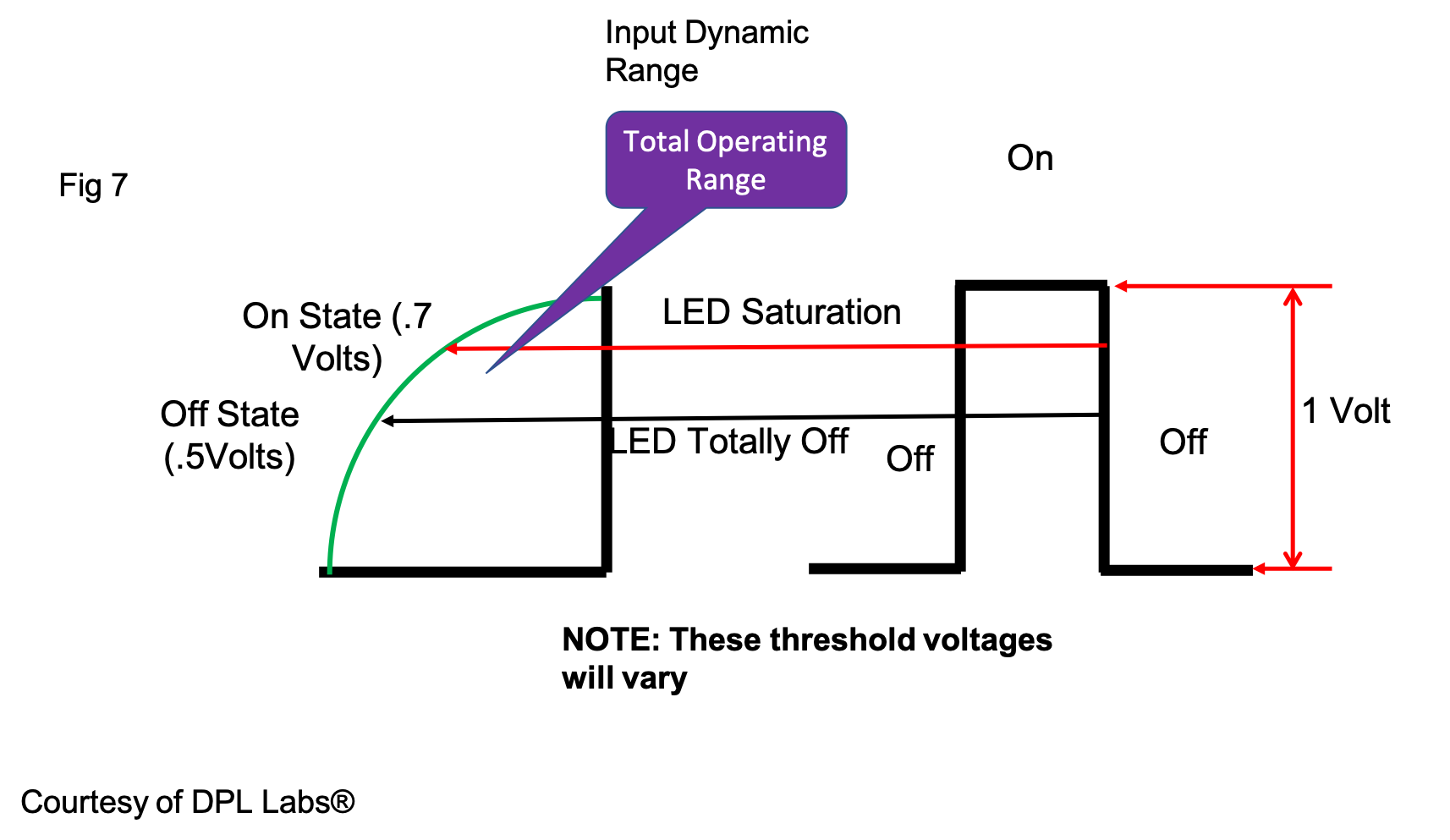

However, one critical area remains: what happens if a signal enters the circuit that may be a bit too low? Figure 9 shows how a small buffer amplifier can be inserted to help ensure the signal registers a solid ON state and OFF state. Even this buffer has limits, characterized as the Input Dynamic Range of the device; it is where standards play such a crucial role in its operation. Figure 10 shows the big picture. Here the input dynamic range is depicted with Vmax and Vmin. The output of this input stage is coupled to a reflective coupler directing light energy into the optical fiber cable. Notice that the input range includes a safe zone where any incoming signal operates dynamically within the device’s limits. However, stepping outside this safe zone can lead to problems rapidly. When streaming trillions of bits per second, it is essential to have a well-established, wide dynamic input range with precise signal ON/OFF states. This error happens far too often.

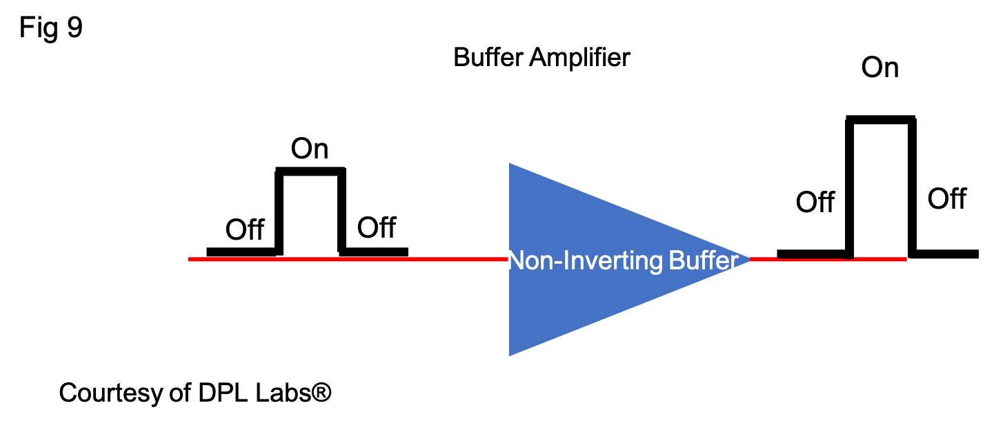
The accompanying waveforms illustrate what these signals can look like under three different conditions. The saturated waveform results in distorted eye patterns with multiple data points that produces errors. Signals that are too low can fall below the input minimums, leading to intermittent capture and interference from the noise floor. Conversely, the normal waveform displays a robust output with minimal distortions and noise.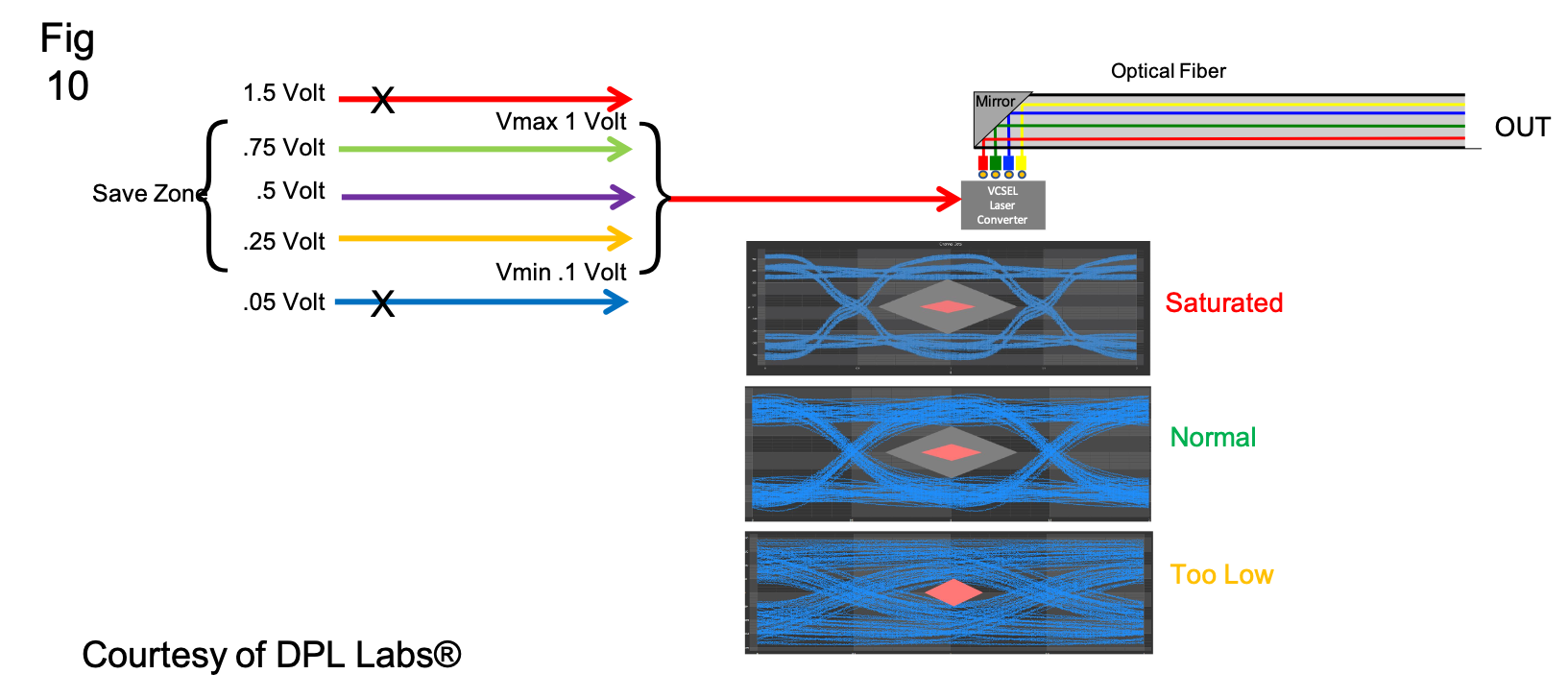

Hybrid Optical Assemblies

Some optical cable assemblies incorporate other multiple connections that perform various other functions within each cable. This is driven by cost considerations or is necessary to provide additional electrical options required by the interface. To discuss this further, we’ll stay focused on consumer video and HDMI, as it is more relevant to this demographic.

HDMI Rev 2.1 Interface

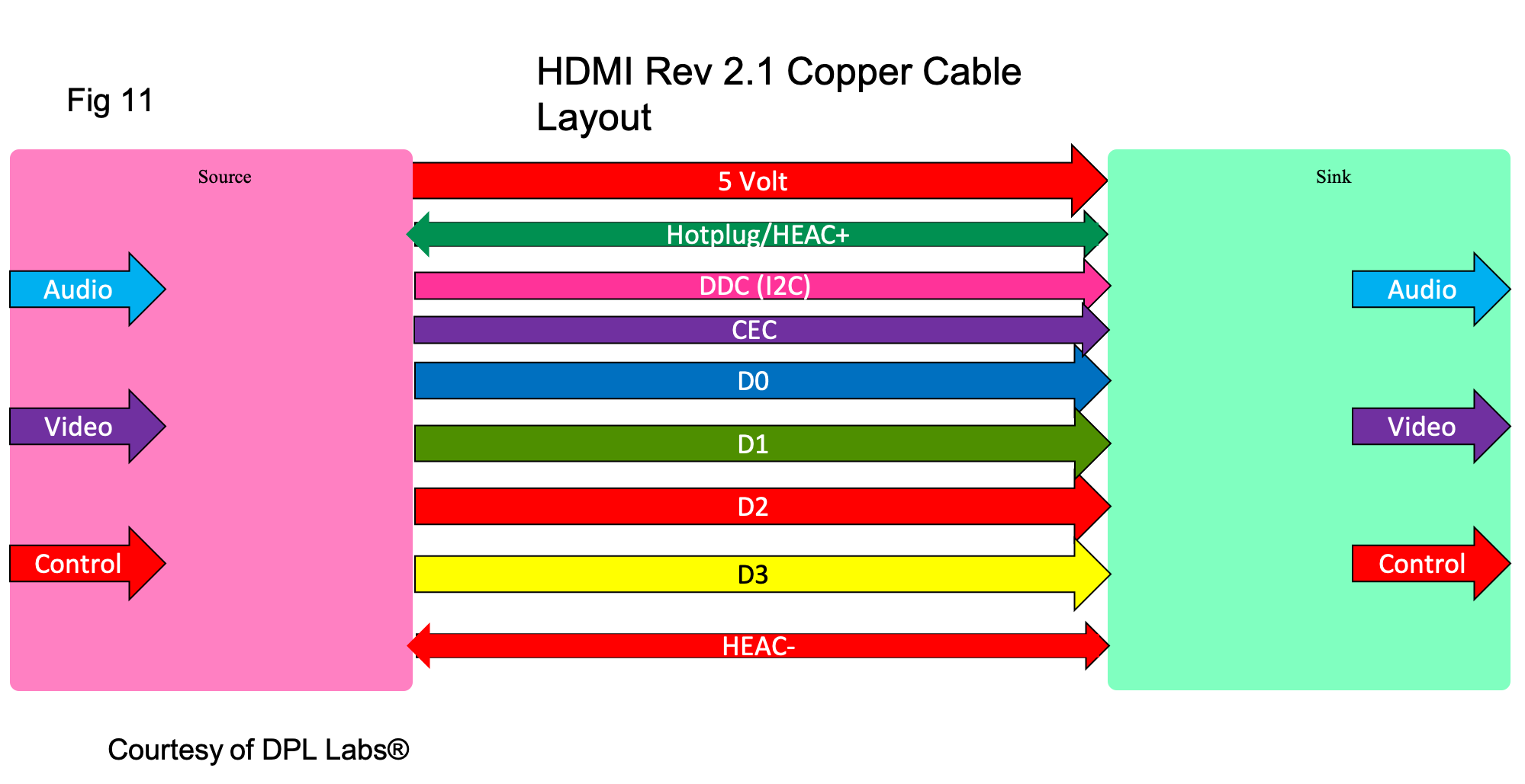
The HDMI interface is a prime example of the need for multiple types of channels. Figure 11 details the components of an HDMI Rev 2.1 copper cable interface, which consists of nine separate channels:

1. DC Voltage: The main source that carries 5 volts DC to the entire interface including a sink device (destination device).

2. HotPlug Detection and HEAC+ (Positive Channel for Internet): Sends a return DC signal back to the source, indicating a connection and starting the telemetry process; also acts as one channel of a 200MHz Ethernet.

3. DDC: Carries all telemetry, such as content protection and screen resolution for the interface. It operates at low data rates of 100KHz and can be susceptible to high capacitive loading, causing data errors that can be corrected to some extent with inexpensive electronics.

4. D0, D1, D2, and D3: Carry high-speed video data.

5. HEAC- (Negative Differential Channel for 200MHz Internet)

6. CEC: Used for incorporating a single remote control and low-level data.

You can see in Figure 12 that out of these nine channels, only four are typically used with optical fiber due to their high-speed data rates (now up to 12GHz). The other five are either low frequency signaling or provide some form of direct current (DC) support to meet the interface requirements. Channels that do not require optical fiber are labeled with a W (indicating they are wired, not fiber).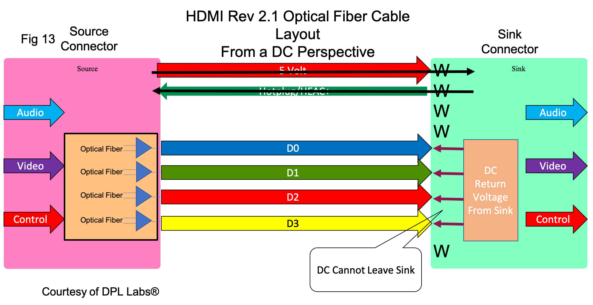

Figure 12 also highlights the channels that must provide direct current (DC) using black arrow identifiers. Since optical fiber cannot conduct DC, copper wires must be used for these channels. You may have already deduced that the HDMI optical fiber configuration shown in Figure 12 would never work.

If you haven’t, let me explain. You may have noticed that all four video channels (D0, D1, D2, D3) requires a critical DC value that must return to the source. As mentioned earlier, optical fiber cannot conduct DC. Without this critical value of voltage that has to stay within 10ths of a volt from specification, the system cannot work. This is where the designer must devise a solution to “fool” the system into operation. Navigating these waters can be treacherous if you don’t fully understand every nuance of the interface.

Figure 13 simplifies the schematic, showing only the wires that must carry the DC component. Here, the remaining six conductors have the task of supporting all the DC functions necessary for the interface to operate.

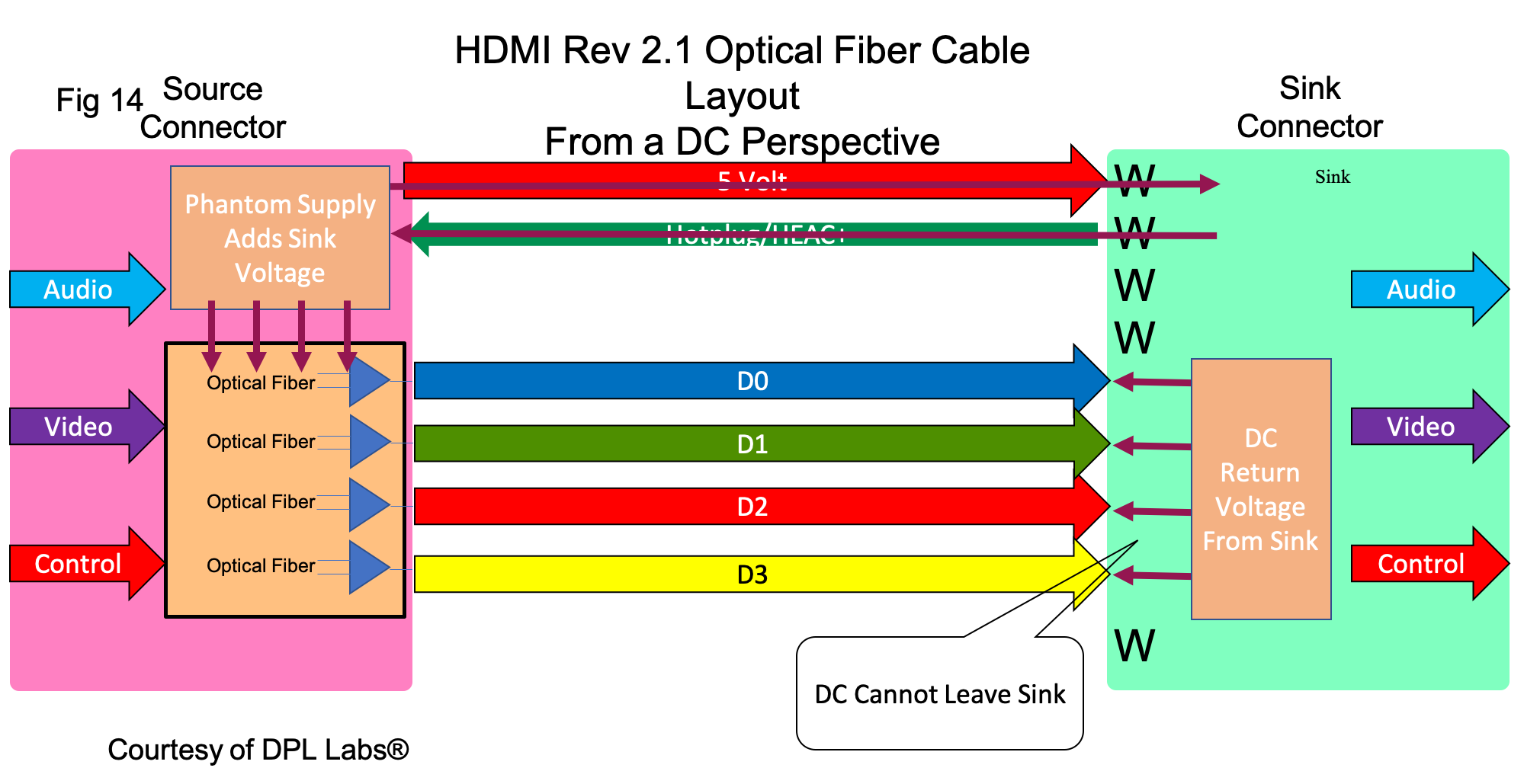It becomes obvious that the return DC channels from the sink have no path back to the source, which is mandatory. So, how is this corrected? Figure 14 shows how additional electronics can be inserted into the source connector’s head-shell to produce a phantom regulated voltage supply, bypassing what the fiber cannot provide.

One must always remember that there are limitations with the main source 5-volt supply located at the source. This supply is not designed to power anything substantial; it is only needed to power up some very low-current devices in the sink (in this case, the display) and Hotplug return. However, by adding an additional Phantom supply we are now asking for more power from the same low-current HDMI source voltage. This is where things can go astray. The specification calls for supply currents greater than 55mA. This means that source devices like Apple TV, set top boxes or AVR’s must at least provide this 55mA current level. Higher currents can be provided, but these specifications are never published by any source. So engineers essentially use the old standby WAG method (Wild Ass Guess). Hmmm, what happened to all these critical values we have been discussing throughout this series?

It gets even more complicated. The already tapped power from the HDMI source is now also required to provide voltage and current to the electronics in the AOC’s sink head-shell. Yep, the light energy produced by the VCSELs have to be converted back to electrical signals again. There is no black magic here. Another set of electronics must be added to the back-sink side of the system to do this conversion. This increases current demands even more, which strains the already weak 5 volt current and can reduce its necessary solid 5 Volts required by the interface, which in turn affects other portions and parts of the interface.

As an example, the DDC channel is always affected by these misguided designs. DDC supply voltage originates from the main 5 volt source. If this voltage drops, so does the DDC rail voltage, changing its response curves, risetime numbers and limiting DDC integrity. Oh, but there is more!

Since the sink reverse voltage is not used due to its now established Phantom supply in the source head shell AOC designers don’t let that go to waste.

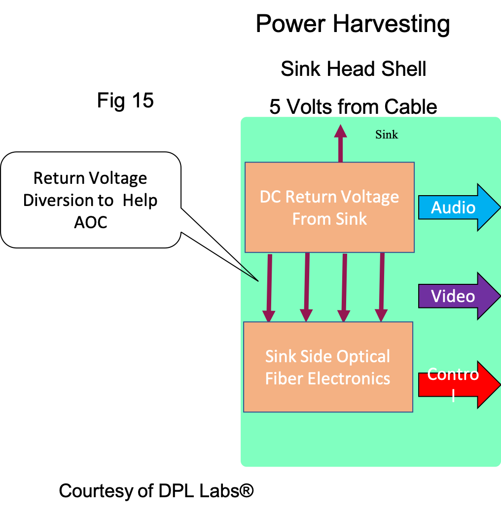Figure 15 illustrates how the sink return voltage is not wasted. Since this voltage is part of the original HDMI specification it is sitting there now doing, optical fiber manufacturers use this now-untapped resource to help power the sink’s optical converter electronics. Referred to as “Power Harvesting,” this increases current demand throughout the entire interface, including the Phantom power source in the source HDMI connector in Figure 14. In addition, as currents go up and source voltages go down, it can spread to areas like the expected “Power Harvesting” we just explained. This vicious cycle is found in the majority of Active Optical Cables. Some work and some don’t. Some work for a week, while others last for a year. The lack of a full understanding of the total impact when guessing leads to poor reliability and performance.

So, what’s the fix for all of this?

It really does not take much to resolve most of these issues!

Dynamic Range Limits

These dynamic range issues can be easily resolved. The key is announcing each AOC’s input dynamic range to its user. Once this is known, the customer or integrator simply has to take the dynamic range limits and match the source device output levels to the cable. Easy, right? Unfortunately, it’s not. Life would be much easier if all products provided these numbers, but the likelihood of transparency is almost ZERO. That means someone else has to do it. How Stupid. We will get into this a little later.

Power Limitations

There are several ways to address these power issues by thinking a bit outside the box:

• Low Source Power: Devices are available that allow users to tap into an HDMI AOC and add additional power via an external power supply. These supplies range from 0.5 amps to as much as 5 amps. However, using high-current devices (5 amps) is not always advisable because the wires within the AOC are relatively small in gauge and can only handle a limited amount of current. A reasonable current value from an external device like this is 1 amp (1000mA).

• More Efficient AOC Devices: Over the past few years, these devices have improved with lower current demands. While they may be a bit more expensive, the benefits clearly outweigh the potential failures. For example, AOC devices from just three years ago typically demanded 160mA to as much as 320mA. Given that the HDMI specification is only 55mA, it’s easy to understand why so many issues can arise. In some cases, the current demand for certain AOC devices were so high it would overheat the supply electronics in the source and die resulting in system failure. Again, this can happen at any time be it from the initial installation to a day, weeks, months, or years later.

What About Fiber Only AOC’s?

Let’s not forget about the optical fiber solutions that use no copper at all, as shown in Figure 16. These generally offer the best reliability and performance but come at substantially higher costs. These are typically one or two-fiber devices and do not resemble traditional cables. Instead, they have a chassis-like design (dongle) with separate power supplies. The copper wires are completely removed, allowing for signal multiplexing for the remainder of the interface. Using these types of products virtually eliminates the issues we have discussed.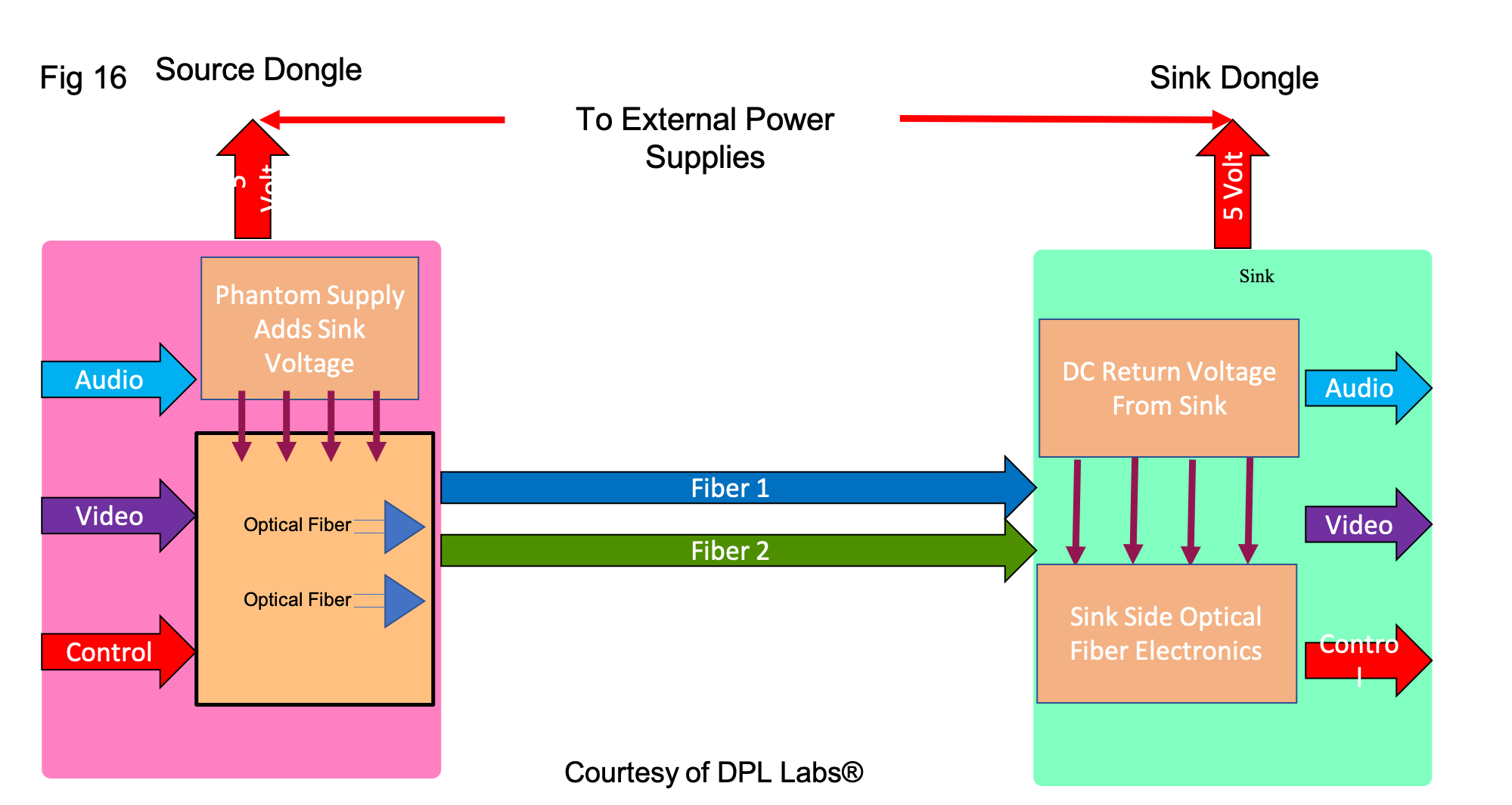

Although copper-free devices have their benefits, they also come with some minor inconveniences, such as managing two chassis and two separate power supplies where space can become an issue. They are also susceptible to High-Speed integrity issues found in many poorly designed devices. However, their advantages far outweigh the relatively small drawbacks.

We still have progress to make with high-performance AOC cables. Their usefulness is undeniable, and with proper safeguards, their reliability and performance can be significantly enhanced, leading to more sustainable high-performance video systems.

Conclusion

Since DPL Labs began testing high-performance cable devices, test limits are continually updated with tighter specifications and procedures. This progress is driven by investigating field failures, similar to what we have just learned, and emulating these exact systems at DPL Labs HQ, verifying each reported issue. Through these case studies, DPL Labs identifies which products fail, why they fail, and how to rectify these failures. This process allows DPL Labs to develop new tests and procedures to identify these potential failures before cable products go into service.

AOC issues are no different. Expecting transparency from manufacturers on these matters is often futile. All AOC products that pass DPL Labs’ stringent testing process must meet specific minimum standards to earn certification. Signal levels are measured and identified, Power consumption is measured to ensure consumers and integrators do not need to worry about the issues we have presented here. Rest assured that all HDMI Optical Fiber products that pass and earn the DPL Labs Reference Standard Certification have performance levels far above typical HDMI standards. Every discovered issue is passed on to our engineering group for updated tests keeping all DPL members at the top of their game.

Should you have any additional questions about this series, feel free to contact DPL Labs directly at info@dpllabs.com.

DPL Labs Certified AOC Products

Where Only the Best Pass the DPL Test